Two-way ANOVA without replication
Manual and Pythonic
By SAJEEWA PEMASINGHE
Two-way ANOVA is used when there are two factors that can influence the result of a measurement.
For example, if four analysts made their measurements of the concentration of lead using the same instrument, determining if there is a significant difference between the data produced by the different analysts would constitute a one-way ANOVA.
If there were three instruments available in the lab, and if each analyst repeated their measurements on all three instruments, now there would be two factors: analyst and the instrument the effects of which have to be separately accounted for.
We can use two-way ANOVA to determine whether either (or both) of the factors have a significant effect on the measurements.
It could also be the case that one factor changes the effect of another. This is known as an interaction. Two-way ANOVA also enables us to find the existence of such possible interactions.
Depending on the experimental design, there can be two flavors of two-way ANOVA:
- factorial (or cross-classified) ANOVA
- hierarchical (or nested) ANOVA
Within factorial ANOVA there are two variations:
- two-way ANOVA without replication
- two-way ANOVA with replication
We are going to focus on two-way ANOVA without replication. For two-way ANOVA without replication, ‘interactions’ (as described previously) are not applicable.
As always, we will look at an example to undestand the calculations and concepets behind two-way ANOVA without replication.
Example:
A new method to determine the amount of low-calorie sweetener in different food samples has been introduced by a company. The company wants to apply this method on four food samples. The company has four labs. So the tests that involve the application of this new method to each of the food samples will be carried out in each of the four labs. Each of the labs have reported the mean recovery percentages of the amount of low-calorie sweetener they could detect on each of the food samples. The data are given below.
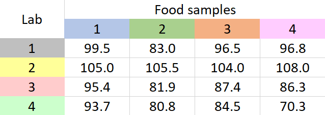
Table 1: Mean recovery percentages for a sweetener in four food samples
It seems that different labs have different results for each sample. What we have to ascertain is if any of these results have occurred due to chance variation. To establish this, we go for two-way ANOVA without replication. Why ‘without replication’? Because from each lab we have only one value for percentage recovery (which is the mean value). If there had been more than one value for percentage recovery from each lab, for each food sample, we would have to go for two-way ANOVA with replication.
Using two-way ANOVA without replication, we are going to calculate the F statisitc for both the groups (i.e. food samples/columns) and the blocks (i.e. labs/rows).
The main equations for two-way ANOVA without replication are given below with the expanded meaning of each term.
SST\quad =\quad SSG\quad +\quad SSB\quad +\quad SSE\quad \quad \quad \quad \quad \quad \quad (1)
{ F }_{ groups }\quad =\quad \large \frac { \left( \frac { SSG }{ { df }_{ groups } } \right) }{ \left( \frac { SSE }{ { df }_{ error } } \right) }\normalsize \quad \quad \quad \quad \quad \quad \quad \quad \quad \quad \quad \quad \quad \quad (2)
{ F }_{ blocks }\quad =\quad \large \frac { \left( \frac { SSB }{ { df }_{ blocks } } \right) }{ \left( \frac { SSE }{ { df }_{ error } } \right) } \normalsize \quad \quad \quad \quad \quad \quad \quad \quad \quad \quad \quad \quad \quad \quad (3)
SST\quad =\quad Sum\quad of\quad squares\quad total
SSG\quad =\quad Sum\quad of\quad squares\quad groups\quad (i.e.\quad columns)
SSB\quad =\quad Sum\quad of\quad squares\quad blocks\quad (i.e.\quad rows)
SSE\quad =\quad Sum\quad of\quad squares\quad error
{ df }_{ groups }\quad =\quad degrees\quad of\quad freedom\quad groups
{ df }_{ blocks }\quad =\quad degrees\quad of\quad freedom\quad blocks
{ df }_{ error }\quad =\quad degrees\quad of\quad freedom\quad error
Calculating { F }_{ groups } and { F }_{ blocks } manually
- Add all the 16 mean recovery values and divide by 16 to get the overall mean, { \mu }_{ TOT }\quad =\quad 92.4
- Find the difference between each of the 16 recovery values and the overall mean, square the differences, and add them up to obtain SST
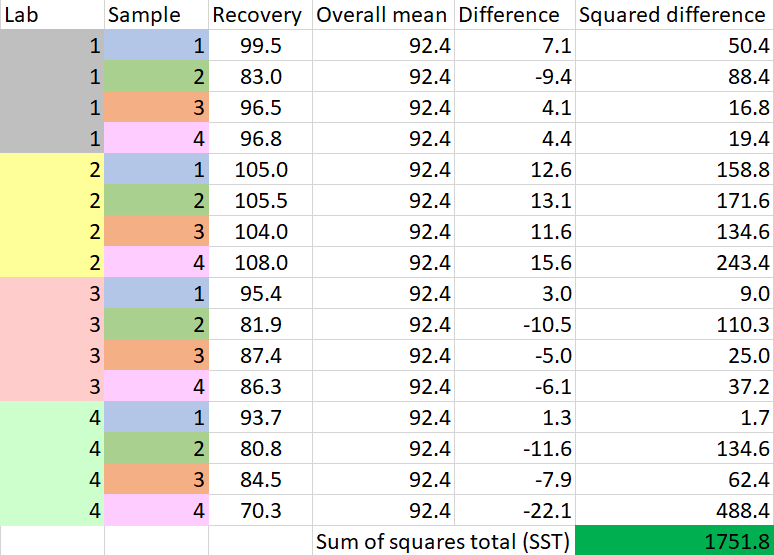
- Find the difference between each group mean and the overall mean, square the differences, add them up, and multiply by the number of items in each group to obtain SSG
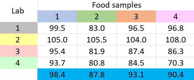
\footnotesize SSG=4\times \left\{ { \left( 98.4-92.4 \right) }^{ 2 }+{ \left( 87.8-92.4 \right) }^{ 2 }+{ \left( 93.1-92.4 \right) }^{ 2 }+{ \left( 90.4-92.4 \right) }^{ 2 } \right\} =247.4
- Find the difference between each block mean and the overall mean, square the differences, add them up, and multiply by the number of items in each group to obtain SSB

\footnotesize SSB=4*\left\{ { \left( 94.0-92.4 \right) }^{ 2 }+{ \left( 105.6-92.4 \right) }^{ 2 }+{ \left( 87.8-92.4 \right) }^{ 2 }+{ \left( 82.3-92.4 \right) }^{ 2 } \right\} =1201.7
- Since we have already calculated SST, SSG, and SSB, we can calculate SSE using equation (1)
SSE=SST-SSG-SSB=302.7
- Calculating degrees of freedom
{ df }_{ groups }=number\quad of\quad groups-1=4-1=3
{ df }_{ blocks }=number\quad of\quad blocks-1=4-1=3
{ df }_{ error }={ df }_{ groups }\times { df }_{ blocks }=3\times 3=9
- Calculating { F }_{ groups } using equation (2)
\large { F }_{ groups }=\frac { \left( \frac { SSG }{ { df }_{ groups } } \right) }{ \left( \frac { SSE }{ { df }_{ error } } \right) } =\frac { \left( \frac { 247.4 }{ 3 } \right) }{ \left( \frac { 302.7 }{ 9 } \right) } =2.452
- Calculating { F }_{ blocks } using equation (3)
\large { F }_{ blocks }=\frac { \left( \frac { SSB }{ { df }_{ blocks } } \right) }{ \left( \frac { SSE }{ { df }_{ error } } \right) } =\frac { \left( \frac { 1201.7 }{ 3 } \right) }{ \left( \frac { 302.7 }{ 9 } \right) } =11.91
Conclusion
Null hypothesis for groups/food samples: { H }_{ 0 }:{ \mu }_{ 1 }={ \mu }_{ 2 }={ \mu }_{ 3 }={ \mu }_{ 4 }
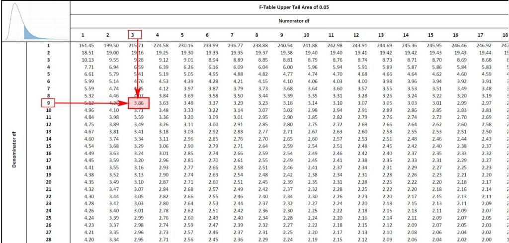
But F_{ groups }=2.452 is smaller than F_{ critical }=3.86. Therefore we cannot reject the null hypothesis which means that there is insufficient evidence to conclude that the recovery depends on the sample type.
Null hypothesis for blocks/labs: { H }_{ 0 }:{ \mu }_{ 1 }={ \mu }_{ 2 }={ \mu }_{ 3 }={ \mu }_{ 4 }
{ F }_{ blocks }=11.91 far exceeds { F }_{ critical }=3.86. Therefore we reject the null hypothesis for the blocks. This means that recoveries for different labs are significantly different at the 95% level of confidence.
Using Python programming language
import numpy as np
import pandas as pd
import statsmodels.api as sm
from statsmodels.formula.api import ols

#create data
df = pd.DataFrame({'Lab': np.repeat(['lab1', 'lab2', 'lab3','lab4'], 4),
                   'Sample': np.tile(np.repeat(['type1', 'type2', 'type3','type4'], 1), 4),
                   'Recovery': [99.5, 83.0, 96.5, 96.8,
                                105.0, 105.5, 104.0, 108.0,
                                95.4, 81.9, 87.4, 86.3,
                                93.7, 80.8, 84.5, 70.3]})

print(df[:])

#perform two-way ANOVA without replication
model = ols('Recovery ~ C(Lab) + C(Sample)', data=df).fit()
print(sm.stats.anova_lm(model, typ=2))
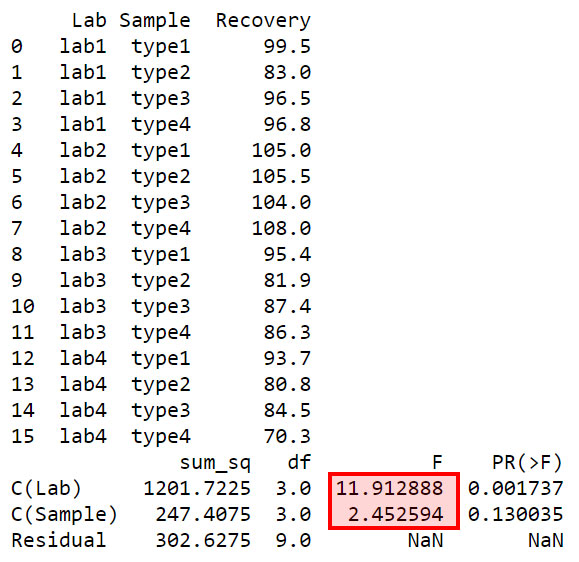
As the above Python output shows, the corresponding P-value for Labs is 0.001737 which is smaller than 0.05. This means, this F value of 11.91 cannot have occurred due to chance at alpha = 0.05. Therefore the recovery values for different labs are significantly different at alpha = 0.05.
For the sample types, the corresponding P-value is 0.130035 which is larger than 0.05. This means that at alpha = 0.05 this F value is not significant (the maximum probability we allow for chance occurrence at alpha = 0.05 is 0.05). As has been stated above, this means that there is insufficient evidence to conclude that the recovery depends on the sample type.
